
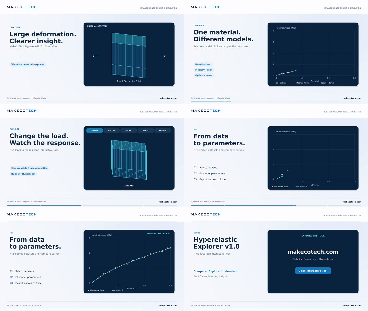
Explore Hyperelastic Explorer in 36 seconds
Compare material models, explore five loading modes, fit experimental data and export curves to Excel.
Why linear elasticity quickly becomes insufficient
Rubber-like materials can look deceptively simple. Pull an elastomeric component and it stretches; release it and, ideally, it returns to its original shape. Mechanically, however, this behavior is very different from the small-strain elasticity commonly used for metals and many structural materials.
For an elastic metal operating below yield, a relationship such as
may describe the response sufficiently well over a limited strain range. For an elastomer undergoing 50%, 100%, or several hundred percent strain, this assumption is no longer appropriate. Geometry changes substantially, the stress-strain response becomes strongly nonlinear, and deformation in one direction is coupled to deformation in the transverse directions.
This is where hyperelastic material models become useful.
From a stress-strain line to a strain-energy function
A hyperelastic material is described through a strain-energy density function. In terms of the principal stretches:
The stresses are then obtained from derivatives of this stored energy. Rather than defining only one nonlinear stress-strain curve, the constitutive law describes how the material stores energy for a complete deformation state.
This framework is particularly useful for elastomers, rubber seals, soft polymers, polymer foams and other materials capable of large approximately reversible deformation.
Why one tensile test is often not enough
A hyperelastic law must describe more than a single uniaxial loading path. Common calibration modes include uniaxial tension, equibiaxial tension, planar tension / pure shear, simple shear and—when compressibility matters—volumetric deformation.
Uniaxial
One principal direction stretches while the transverse directions contract.
Equibiaxial
Two principal directions stretch simultaneously, strongly constraining large-strain behavior.
Planar / Pure Shear
One direction stretches while another direction remains constrained.
Simple Shear
A different deformation path that can expose behavior not visible in uniaxial testing.
For compressible materials, the volume ratio J becomes another independent part of the constitutive response.
Two material models can fit the same uniaxial data well and still predict very different biaxial, shear or volumetric behavior. Hyperelastic calibration should therefore be treated as constitutive-model identification, not simply curve fitting.
The constitutive model changes the prediction
There is no universal hyperelastic law that is best for every material and every deformation range. Simpler models require fewer coefficients; richer models can reproduce more complex nonlinear behavior but demand sufficient experimental information to identify their parameters reliably.
Neo-Hookean
A useful baseline with one deviatoric stiffness parameter.
Mooney–Rivlin
Introduces dependence on both the first and second deviatoric strain invariants.
Ogden
For the one-term Abaqus-style normalization used by the interactive tool:
The parameter μ governs the initial shear stiffness while α strongly influences the nonlinear shape.
| Model in MakeCoTech Hyperelastic Explorer | Main parameters | Typical motivation |
|---|---|---|
| Neo-Hookean | μ | Simple baseline response |
| Mooney–Rivlin | C10, C01 | Two-invariant response |
| Ogden, 1-term | μ, α | Flexible stretch-based nonlinearity |
| Arruda–Boyce | μ, λm | Chain-locking-type behavior |
| Yeoh | C10, C20, C30 | Higher-order first-invariant response |
| Reduced Polynomial N=2 | C10, C20 | Compact higher-order formulation |
| Van der Waals / Kilian | μ, λm, a, β | Flexible network-type response |
| Ogden Hyperfoam N=1 | μ1, α1, ν1 | Highly compressible cellular materials |
Compressibility should not be treated as a secondary detail
Dense elastomers are frequently modeled as nearly incompressible:
For many applications this is a good approximation. But it is not appropriate for every rubber-like material. Foams, for example, can undergo substantial volume change because of their cellular structure.
For several conventional Abaqus hyperelastic models, compressibility is introduced through a separate volumetric parameter such as D1:
Ogden Hyperfoam is different
Hyperfoam is inherently compressible and couples volumetric and distortional response in the same potential. For the one-term formulation implemented in the tool:
This makes Hyperfoam especially relevant when large volume changes are physically expected rather than treated as a small numerical correction.
Where hyperelasticity appears in real products
Seals & O-rings
Contact pressure, assembly squeeze, leakage risk and large local deformation.
Semiconductor Equipment
Vacuum seals, compliant interfaces, isolation elements and polymer components.
Foams
Large compression with substantial volumetric deformation.
Medical & Soft Structures
Soft polymers, compliant devices and biological-material approximations.
Automotive
Bushings, mounts, couplings, tires and flexible sealing systems.
General Polymer Design
Highly deformable interfaces, damping elements and flexible products.
For a sealing problem, the engineering question is rarely just “how much does it move?” Contact pressure, local strain, compressibility, friction, temperature and extrapolation of the constitutive law may all influence the result.
What can the experiment actually identify?
More fitting coefficients do not automatically mean more information about the material. For incompressible Mooney–Rivlin behavior in simple shear:
and therefore
Simple-shear data can identify the sum C10 + C01, but not the two coefficients independently. Planar deformation has a similar limitation. Additional independent deformation modes such as uniaxial or biaxial data are needed to separate them.
An optimizer can always return numbers. The more important question is whether the experimental program contains enough independent information for those numbers to be meaningful.
Making nonlinear constitutive behavior easier to “feel”
Hyperelastic laws are often presented as equations and coefficient tables. An engineer may receive a parameter set such as
or
without immediately developing an intuitive understanding of how those values change the material response.
That motivated the development of MakeCoTech Hyperelastic Explorer v1.0: an interactive engineering environment in which the constitutive law can be explored before geometry, contact, meshing and solver settings are added to the problem.
MakeCoTech Hyperelastic Explorer v1.0
The tool compares nonlinear material laws, visualizes stress and stored energy while deformation is changed interactively, accepts multi-mode experimental datasets, performs material fitting, includes Abaqus-oriented benchmark datasets and exports the resulting curves and parameters to Excel.
Reference name: MakeCoTech Hyperelastic Explorer v1.0, MakeCoTech, 2026.
Checking the fitting workflow against Abaqus examples
The tool provides two examples with distinct purposes:
Hyperelastic benchmark: Abaqus SI Hypertest
Published rubber data for uniaxial, biaxial, planar and volumetric loading, used to explore deviatoric fitting and compressibility.
Hyperfoam demonstration
Synthetic one-term Ogden Hyperfoam data across five loading modes, generated with μ₁ = 0.5 MPa, α₁ = 2 and ν₁ = 0.20 to demonstrate parameter fitting.
The Hyperfoam example uses generated model data. It demonstrates the fitting workflow and requires separate experimental or solver data for external validation.
A good fit is not the end of the engineering work
A parameter set can reproduce measured data closely and still behave poorly when extrapolated. Pure hyperelasticity also does not automatically represent rate dependence, hysteresis, Mullins softening, permanent deformation, temperature dependence or damage.
Educational and preliminary engineering use. MakeCoTech Hyperelastic Explorer is intended for learning, constitutive-model exploration and preliminary calibration. Fitted coefficients and extrapolated behavior must be independently verified before design, safety-critical calculations or production finite element analysis. MakeCoTech provides no warranty for the suitability of a fitted material law in a particular application.
From equations to engineering intuition
The motivation behind the tool is to move from
toward a more transparent workflow:
When the material law is explored independently, it becomes easier to ask the questions that matter: Why do two fitted models diverge in another loading mode? Is a parameter actually identifiable? How much volume change is predicted? What happens beyond the experimental range?
Benchmark and formulation references
Abaqus / SIMULIA, Hyperelastic Behavior of Rubberlike Materials.
SIMULIA hyperelastic material documentation
Abaqus / SIMULIA, Rubber under uniaxial tension — hyperelastic benchmark.
SIMULIA SI hyperelastic benchmark
Abaqus 2016 Benchmarks Guide, Fitting of rubber test data.